Dimensionality Reduction

Contents

Main Approaches for Dimensionality Reduction

• Projection
• Manifold

Projection

In most real-world problems, training instances are not spread out uniformly across all dimensions. Many features are almost constant, while others are highly correlated. As a result, all training instances actually lie within (or close to) a much lower-dimensional subspace of the high-dimensional space.

Explaining beyond this more clearly requires more reading of this topic.

i hope the images help a bit.

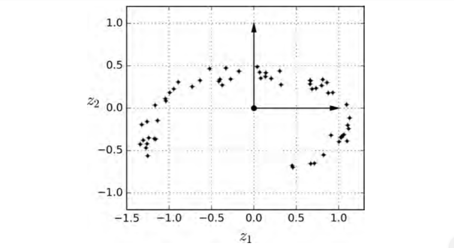
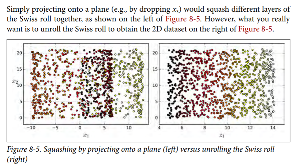
we took a dataset and found that this can be squashed into a hyperplane with no change in interpretation of data.

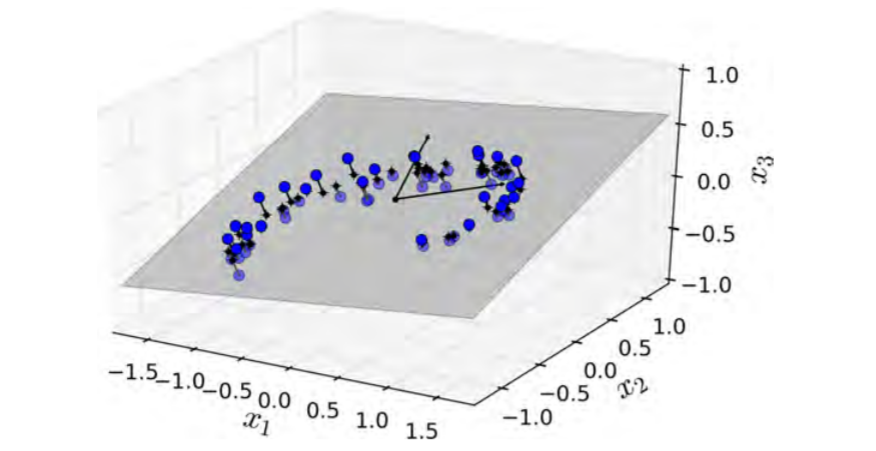
Projected Dataset Plot

However this doesnt always work as we see in this following example

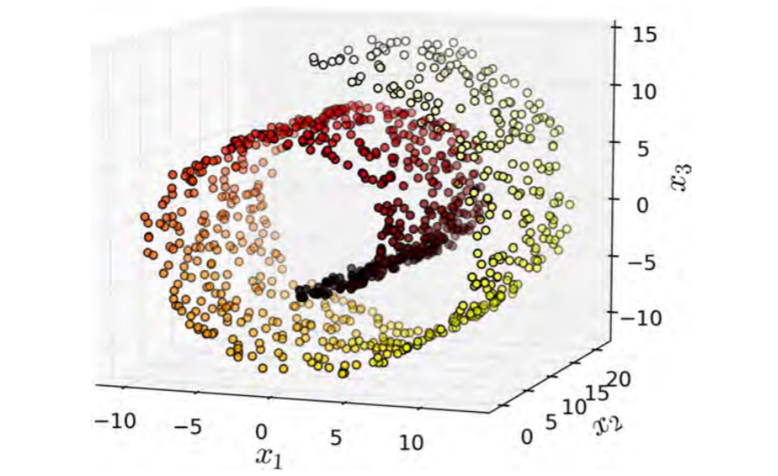
Manifold Learning

The Swiss roll is an example of a 2D manifold. Put simply, a 2D manifold is a 2D shape that can be bent and twisted in a higher-dimensional space. More generally, a d-dimensional manifold is a part of an n-dimensional space (where d < n) that locally resembles a d-dimensional hyperplane. In the case of the Swiss roll, d = 2 and n = 3: it locally resembles a 2D plane, but it is rolled in the third dimension. Many dimensionality reduction algorithms work by modeling the manifold on which the training instances lie; this is called Manifold Learning. It relies on the manifold assumption, also called the manifold hypothesis, which holds that most real-world high-dimensional datasets lie close to a much lower-dimensional manifold. This assumption is very often empirically observed.

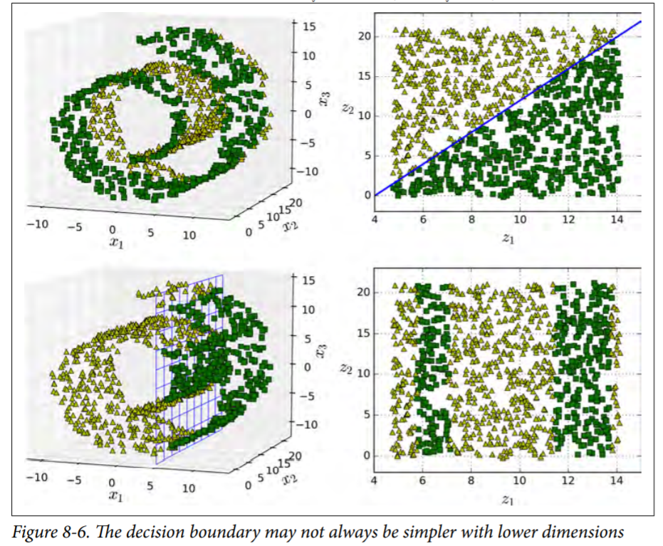
"The manifold assumption is often accompanied by another implicit assumption: that the task at hand (e.g., classification or regression) will be simpler if expressed in the lower-dimensional space of the manifold. For example, in the top row of Figure 8-6 the Swiss roll is split into two classes: in the 3D space (on the left), the decision boundary would be fairly complex, but in the 2D unrolled manifold space (on the right), the decision boundary is a simple straight line. However, this assumption does not always hold. For example, in the bottom row of Figure 8-6, the decision boundary is located at x1 = 5. This decision boundary looks very simple in the original 3D space (a vertical plane), but it looks more complex in the unrolled manifold (a collection of four independent line segments). In short, if you reduce the dimensionality of your training set before training a model, it will definitely speed up training, but it may not always lead to a better or simpler solution; it all depends on the dataset. Hopefully you now have a good sense of what the curse of dimensionality is and how dimensionality reduction algorithms can fight it, especially when the manifold assumption holds. The rest of this chapter will go through some of the most popular algorithms."

See Figure for a better idea

As of now even I have hard time understanding this and further reading on this will help in getting a more clearer ides

PCA - Principal Component Analysis

First it identifies the hyperplane that lies closest to the data, and then it projects the data onto it.

Preserving Variance

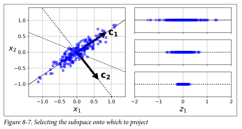
Before you can project the training set onto a lower-dimensional hyperplane, you first need to choose the right hyperplane. For example, a simple 2D dataset is repre‐ sented on the left of Figure 8-7, along with three different axes (i.e., one-dimensional hyperplanes). On the right is the result of the projection of the dataset onto each of these axes. As you can see, the projection onto the solid line preserves the maximum variance, while the projection onto the dotted line preserves very little variance, and the projection onto the dashed line preserves an intermediate amount of variance.

It seems reasonable to select the axis that preserves the maximum amount of var‐ iance, as it will most likely lose less information than the other projections. Another way to justify this choice is that it is the axis that minimizes the mean squared dis‐ tance between the original dataset and its projection onto that axis. This is the rather simple idea behind PCA.

Principal Components

PCA identifies the axis that accounts for the largest amount of variance in the train‐ ing set. In Figure 8-7, it is the solid line. It also finds a second axis, orthogonal to the first one, that accounts for the largest amount of remaining variance. In this 2D example there is no choice: it is the dotted line. If it were a higher-dimensional data‐ set, PCA would also find a third axis, orthogonal to both previous axes, and a fourth, a fifth, and so on—as many axes as the number of dimensions in the dataset.

The direction of the principal components is not stable: if you per‐ turb the training set slightly and run PCA again, some of the new PCs may point in the opposite direction of the original PCs. How‐ ever, they will generally still lie on the same axes. In some cases, a pair of PCs may even rotate or swap, but the plane they define will generally remain the same.

So how can you find the principal components of a training set? Luckily, there is a standard matrix factorization technique called Singular Value Decomposition (SVD) that can decompose the training set matrix X into the matrix multiplication of three matrices

$U.Σ.V^T$

X_centered = X - X.mean(axis=0)
U, s, Vt = np.linalg.svd(X_centered)
c1 = Vt.T[:, 0]
c2 = Vt.T[:, 1]

Projecting Down to d Dimensions

Once you have identified all the principal components, you can reduce the dimen‐ sionality of the dataset down to d dimensions by projecting it onto the hyperplane defined by the first d principal components. Selecting this hyperplane ensures that the projection will preserve as much variance as possible.

To project the training set onto the hyperplane, you can simply compute the matrix multiplication of the training set matrix X by the matrix Wd , defined as the matrix containing the first d principal components (i.e., the matrix composed of the first d columns of V)

$X_{d‐proj} = X.W_d$

PCA assumes that the dataset is centered around the origin. As we will see, Scikit-Learn’s PCA classes take care of centering the data for you. However, if you implement PCA yourself (as in the pre‐ ceding example), or if you use other libraries, don’t forget to center the data first.

Scikit-Learn

from sklearn.decomposition import PCA
pca = PCA(n_components = 2)
X2D = pca.fit_transform(X)

Exaplained Variance Ratio

Exaplained Variance Ratio indicates the proportion of the dataset’s variance that lies along the axis of each principal component.

>>> pca.explained_variance_ratio_
array([0.84248607, 0.14631839])

This tells you that 84.2% of the dataset’s variance lies along the first axis, and 14.6% lies along the second axis. This leaves less than 1.2% for the third axis, so it is reason‐ able to assume that it probably carries little information.

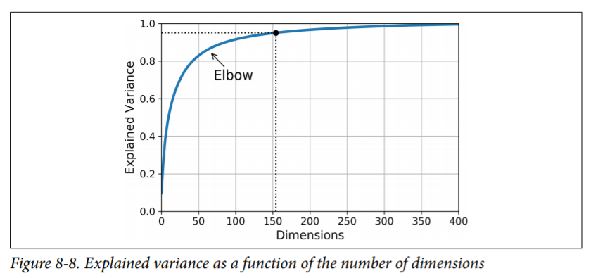
Choosing the Right Number of Dimensions

Instead of arbitrarily choosing the number of dimensions to reduce down to, it is generally preferable to choose the number of dimensions that add up to a sufficiently large portion of the variance (e.g., 95%). Unless, of course, you are reducing dimen‐ sionality for data visualization—in that case you will generally want to reduce the dimensionality down to 2 or 3.

pca = PCA(n_components=0.95)
X_reduced = pca.fit_transform(X_train)

how to find number of dimensions

pca = PCA()
pca.fit(X_train)
cumsum = np.cumsum(pca.explained_variance_ratio_)
d = np.argmax(cumsum >= 0.95) + 1

PCA for Compression

Try applying PCA to the MNIST dataset while preserving 95% of its var‐ iance. You should find that each instance will have just over 150 features, instead of the original 784 features. So while most of the variance is preserved, the dataset is now less than 20% of its original size! This is a reasonable compression ratio, and you can see how this can speed up a classification algorithm (such as an SVM classifier) tremendously. It is also possible to decompress the reduced dataset back to 784 dimensions by applying the inverse transformation of the PCA projection. Of course this won’t give you back the original data, since the projection lost a bit of information (within the 5% variance that was dropped), but it will likely be quite close to the original data. The mean squared distance between the original data and the reconstructed data (compressed and then decompressed) is called the reconstruction error.

pca = PCA(n_components = 154)
X_reduced = pca.fit_transform(X_train)
X_recovered = pca.inverse_transform(X_reduced)

$X_{recovered} = X_{d‐proj}.W_d ^T$

Randomized PCA

If you set the svd_solver hyperparameter to "randomized", Scikit-Learn uses a sto‐ chastic algorithm called Randomized PCA that quickly finds an approximation of the first d principal components. Its computational complexity is $O(m × d^2) + O(d^3)$, instead of $O(m × n^2) + O(n^3)$ for the full SVD approach, so it is dramatically faster than full SVD when d is much smaller than n:

rnd_pca = PCA(n_components=154, svd_solver="randomized")
X_reduced = rnd_pca.fit_transform(X_train)

Incremental PCA

One problem with the preceding implementations of PCA is that they require the whole training set to fit in memory in order for the algorithm to run. Fortunately, Incremental PCA (IPCA) algorithms have been developed: you can split the training set into mini-batches and feed an IPCA algorithm one mini-batch at a time.

The following code splits the MNIST dataset into 100 mini-batches (using NumPy’s array_split() function) and feeds them to Scikit-Learn’s IncrementalPCA class5 to reduce the dimensionality of the MNIST dataset down to 154 dimensions (just like before).

from sklearn.decomposition import IncrementalPCA
n_batches = 100
inc_pca = IncrementalPCA(n_components=154)
for X_batch in np.array_split(X_train, n_batches):
 inc_pca.partial_fit(X_batch)
X_reduced = inc_pca.transform(X_train)

Alternatively, you can use NumPy’s memmap class, which allows you to manipulate a large array stored in a binary file on disk as if it were entirely in memory; the class loads only the data it needs in memory, when it needs it. Since the IncrementalPCA class uses only a small part of the array at any given time, the memory usage remains under control. This makes it possible to call the usual fit() method, as you can see in the following code:

X_mm = np.memmap(filename, dtype="float32", mode="readonly", shape=(m, n))
batch_size = m // n_batches
inc_pca = IncrementalPCA(n_components=154, batch_size=batch_size)
inc_pca.fit(X_mm)

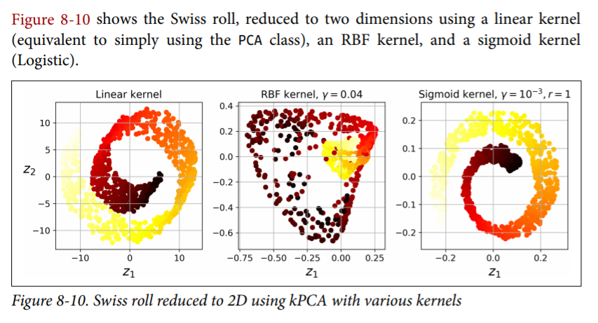
Kernal PCA

Kernel Trick can be applied to PCA making it possible to perform complex nonlinear projections for dimensionality redution. This is called KernelPCA or KPCA.

It is often good at preserving clusters of instances after projection, or sometimes even unrolling datasets that lie close to a twisted manifold.

from sklearn.decomposition import KernelPCA
rbf_pca = KernelPCA(n_components = 2, kernel="rbf", gamma=0.04)
X_reduced = rbf_pca.fit_transform(X)

Selecting a Kernel and Tuning Hyperparameters

As kPCA is an unsupervised learning algorithm, there is no obvious performance measure to help you select the best kernel and hyperparameter values. However, dimensionality reduction is often a preparation step for a supervised learning task (e.g., classification), so you can simply use grid search to select the kernel and hyper‐ parameters that lead to the best performance on that task.

For example, the following code creates a two-step pipeline, first reducing dimensionality to two dimensions using kPCA, then applying Logistic Regression for classification. Then it uses Grid SearchCV to find the best kernel and gamma value for kPCA in order to get the best classification accuracy at the end of the pipeline:

from sklearn.model_selection import GridSearchCV
from sklearn.linear_model import LogisticRegression
from sklearn.pipeline import Pipeline

clf = Pipeline([
 ("kpca", KernelPCA(n_components=2)),
 ("log_reg", LogisticRegression())
 ])
param_grid = [{
 "kpca__gamma": np.linspace(0.03, 0.05, 10),
 "kpca__kernel": ["rbf", "sigmoid"]
 }]
grid_search = GridSearchCV(clf, param_grid, cv=3)
grid_search.fit(X, y)

>>> print(grid_search.best_params_)
{'kpca__gamma': 0.043333333333333335, 'kpca__kernel': 'rbf'}

Another approach, this time entirely unsupervised, is to select the kernel and hyperparameters that yield the lowest reconstruction error.

You may be wondering how to perform this reconstruction. One solution is to train a supervised regression model, with the projected instances as the training set and the original instances as the targets. Scikit-Learn will do this automatically if you set fit_inverse_transform=True, as shown in the following code:

rbf_pca = KernelPCA(n_components = 2, kernel="rbf", gamma=0.0433,
 fit_inverse_transform=True)
X_reduced = rbf_pca.fit_transform(X)
X_preimage = rbf_pca.inverse_transform(X_reduced)

By default, fit_inverse_transform=False and KernelPCA has no inverse_transform() method. This method only gets created when you set fit_inverse_transform=True

You can then compute the reconstruction pre-image error:

>>> from sklearn.metrics import mean_squared_error
>>> mean_squared_error(X, X_preimage)
32.786308795766132

Now you can use grid search with cross-validation to find the kernel and hyperpara‐ meters that minimize this pre-image reconstruction error.

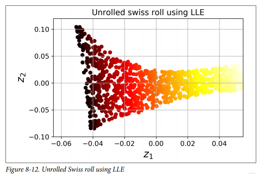
LLE - Locally Linear Embedding

It is a Manifold Learning technique that does not rely on projections like the previous algorithms. In a nutshell, LLE works by first measuring how each training instance linearly relates to its closest neighbors (c.n.), and then looking for a low-dimensional representation of the training set where these local relationships are best preserved (more details shortly). This makes it particularly good at unrolling twisted manifolds, especially when there is not too much noise.

from sklearn.manifold import LocallyLinearEmbedding
lle = LocallyLinearEmbedding(n_components=2, n_neighbors=10)
X_reduced = lle.fit_transform(X)

Equation 8-4. LLE step 1: linearly modeling local relationships

$\hat{W} = argmin_W \sum_{i=1}^{m} (x^{(i)}-\sum_{j=1}^{m} w_{i,j}x^{(j)})^2$

subject to $w_i, j = 0 $ if
$x^j$ is not one of the k c.n. of $x^i$

and

$\sum_(j = 1)^m w_{i, j} = 1 for i = 1, 2, ⋯, m$

Equation 8-5. LLE step 2: reducing dimensionality while preserving relationships

$\hat{Z} = argmin_Z \sum_{i=1}^m ( z^{(i)} - \sum_{j=1}^m \hat{w}_{i,j} z^{(j)} )^2$

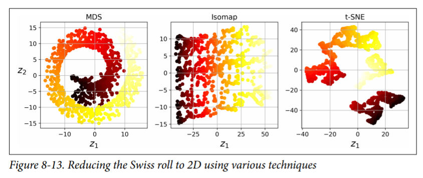
Other Dimensionality Reduction Techniques

• Multidimensional Scaling (MDS) reduces dimensionality while trying to preserve the distances between the instances
• Isomap creates a graph by connecting each instance to its nearest neighbors, then reduces dimensionality while trying to preserve the geodesic distances9 between the instances
• t-Distributed Stochastic Neighbor Embedding (t-SNE) reduces dimensionality while trying to keep similar instances close and dissimilar instances apart. It is mostly used for visualization, in particular to visualize clusters of instances in high-dimensional space (e.g., to visualize the MNIST images in 2D).
• Linear Discriminant Analysis (LDA) is actually a classification algorithm, but during training it learns the most discriminative axes between the classes, and these axes can then be used to define a hyperplane onto which to project the data. The benefit is that the projection will keep classes as far apart as possible, so LDA is a good technique to reduce dimensionality before running another classification algorithm such as an SVM classifier