Training Models 2
Voting Classifier
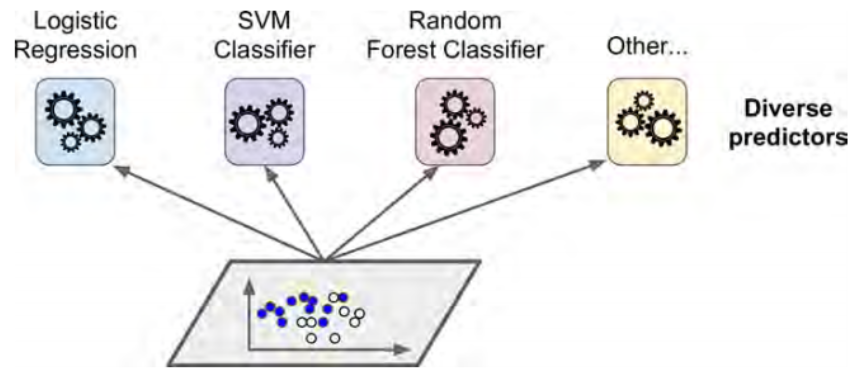
If we have multiple classifiers each acheiving some accuracy and we want to create an even better classifier we use the voting classifier to predict based on predictions of our previously trained classifiers. I hope this image explains this in a better way.
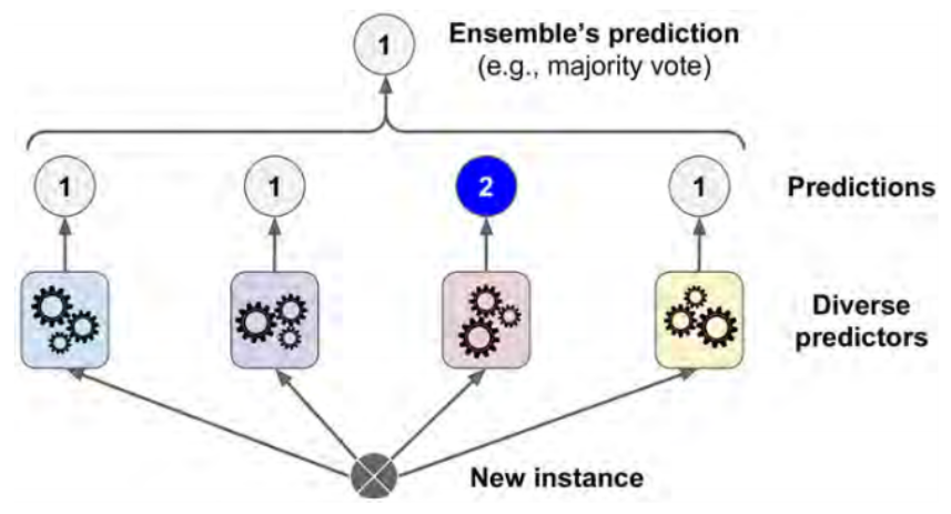
Hard Voting Classifier
Ensemble methods work best when the predictors are as independ‐ ent from one another as possible. One way to get diverse classifiers is to train them using very different algorithms. This increases the chance that they will make very different types of errors, improving the ensemble’s accuracy
Sklearn Example
from sklearn.ensemble import RandomForestClassifier
from sklearn.ensemble import VotingClassifier
from sklearn.linear_model import LogisticRegression
from sklearn.svm import SVC
log_clf = LogisticRegression()
rnd_clf = RandomForestClassifier()
svm_clf = SVC()
voting_clf = VotingClassifier(
 estimators=[('lr', log_clf), ('rf', rnd_clf), ('svc', svm_clf)],
 voting='hard'
 )
voting_clf.fit(X_train, y_train)
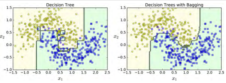
Bagging vs Pasting
Another approach is to use the same training algorithm for every predictor, but to train them on different random subsets of the training set.
When sampling is performed with replacement, this method is called bagging (short for bootstrap aggregating ).
When sampling is performed without replacement, it is called pasting.
In other words, both bagging and pasting allow training instances to be sampled several times across multiple predictors, but only bagging allows training instances to be sampled several times for the same predictor.
Code Example for bagging
to use pasting just set bootstrap = False
from sklearn.ensemble import BaggingClassifier
from sklearn.tree import DecisionTreeClassifier
bag_clf = BaggingClassifier(
 DecisionTreeClassifier(), n_estimators=500,
 max_samples=100, bootstrap=True, n_jobs=-1
 )
bag_clf.fit(X_train, y_train)
y_pred = bag_clf.predict(X_test)
The BaggingClassifier automatically performs soft voting instead of hard voting if the base classifier can estimate class probabilities (i.e., if it has a predict_proba() method), which is the case with Decision Trees classifiers.
Use Out-Of-Bag Evaluation for classification for BaggingClassifier.
Out Of Bag Evolution
With bagging, some instances may be sampled several times for any given predictor, while others may not be sampled at all. By default a BaggingClassifier samples m training instances with replacement (bootstrap=True), where m is the size of the training set. This means that only about 63% of the training instances are sampled on average for each predictor.6 The remaining 37% of the training instances that are not sampled are called out-of-bag (oob) instances. Note that they are not the same 37% for all predictors. Since a predictor never sees the oob instances during training, it can be evaluated on these instances, without the need for a separate validation set. You can evaluate the ensemble itself by averaging out the oob evaluations of each predictor.
bag_clf.oob_score_
Random Patches and Random Subspaces
we can sample features as well.Thus, training each predictor on a random subset of the input features
The BaggingClassifier class supports sampling the features as well. This is con‐ trolled by two hyperparameters: max_features and bootstrap_features. They work the same way as max_samples and bootstrap, but for feature sampling instead of instance sampling. Thus, each predictor will be trained on a random subset of the input features. This is particularly useful when you are dealing with high-dimensional inputs (such as images). Sampling both training instances and features is called the Random Patches method. Keeping all training instances (i.e., bootstrap=False and max_sam ples=1.0) but sampling features (i.e., bootstrap_features=True and/or max_fea tures smaller than 1.0) is called the Random Subspaces method.
Random Forest
Random Forest is an ensemble of Decision Trees, generally trained via the bagging method (or sometimes pasting), typically with max_samples set to the size of the training set. Instead of building a BaggingClassifier and passing it a DecisionTreeClassifier, you can instead use the RandomForestClassifier class, which is more convenient and optimized for Decision Trees (similarly, there is a RandomForestRegressor class for regression tasks).
Read About ExtraTreesClassifier
It is hard to tell in advance whether a RandomForestClassifier will perform better or worse than an ExtraTreesClassifier. Generally, the only way to know is to try both and compare them using cross-validation (and tuning the hyperparameters using grid search).
Feature Importance
In a single Decision Tree, important features are likely to appear closer to the root of the tree, while unimportant features will often appear closer to the leaves (or not at all). It is therefore possible to get an estimate of a feature’s importance by computing the average depth at which it appears across all trees in the forest. Scikit-Learn computes this automatically for every feature after training. You can access the result using the featureimportances variable
>>> from sklearn.datasets import load_iris
>>> iris = load_iris()
>>> rnd_clf = RandomForestClassifier(n_estimators=500, n_jobs=-1)
>>> rnd_clf.fit(iris["data"], iris["target"])
>>> for name, score in zip(iris["feature_names"], rnd_clf.feature_importances_):
>>> print(name, score)
sepal length (cm) 0.112492250999
sepal width (cm) 0.0231192882825
petal length (cm) 0.441030464364
petal width (cm) 0.423357996355
Random Forests are very handy to get a quick understanding of what features actually matter, in particular if you need to perform feature selection.
Boosting
Boosting (originally called hypothesis boosting) refers to any Ensemble method that can combine several weak learners into a strong learner. Most Popular Boosting methods are :
- AdaBoost(Adaptive Boosting)
- Gradient Boosting
AdaBoost
In an AdaBoost classifier, a first base classifier (such as a Decision Tree) is trained and used to make predictions on the training set. The relative weight of misclassified training instances is then increased. A second classifier is trained using the updated weights and again it makes predictions on the training set, weights are updated, and so on.
There is one important drawback to this sequential learning techni‐ que: it cannot be parallelized (or only partially), since each predic‐ tor can only be trained after the previous predictor has been trained and evaluated. As a result, it does not scale as well as bag‐ ging or pasting.
Mathematical Theory related to AdaBoost could be added here.
Scikit-Learn actually uses a multiclass version of AdaBoost called SAMME (which stands for Stagewise Additive Modeling using a Multiclass Exponential loss function). When there are just two classes, SAMME is equivalent to AdaBoost. Moreover, if the predictors can estimate class probabilities (i.e., if they have a predict_proba() method), Scikit-Learn can use a variant of SAMME called SAMME.R (the R stands for “Real”), which relies on class probabilities rather than predictions and generally performs better
from sklearn.ensemble import AdaBoostClassifier
ada_clf = AdaBoostClassifier(
 DecisionTreeClassifier(max_depth=1), n_estimators=200,
 algorithm="SAMME.R", learning_rate=0.5
 )
ada_clf.fit(X_train, y_train)
If your AdaBoost ensemble is overfitting the training set, you can try reducing the number of estimators or more strongly regulariz‐ ing the base estimator.
Gradient Boosting
Just like AdaBoost, Gradient Boosting works by sequentially adding predictors to an ensemble, each one correcting its predecessor. However, instead of tweaking the instance weights at every iteration like AdaBoost does, this method tries to fit the new predictor to the residual errors made by the previous predictor
Very simple example to understand how Gradient Boosting works
Let’s go through a simple regression example using Decision Trees as the base predic‐ tors (of course Gradient Boosting also works great with regression tasks). This is called Gradient Tree Boosting, or Gradient Boosted Regression Trees (GBRT). First, let’s fit a DecisionTreeRegressor to the training set (for example, a noisy quadratic train‐ ing set):
from sklearn.tree import DecisionTreeRegressor
tree_reg1 = DecisionTreeRegressor(max_depth=2)
tree_reg1.fit(X, y)
Now train a second DecisionTreeRegressor on the residual errors made by the first predictor:
y2 = y - tree_reg1.predict(X)
tree_reg2 = DecisionTreeRegressor(max_depth=2)
tree_reg2.fit(X, y2)
Then we train a third regressor on the residual errors made by the second predictor:
y3 = y2 - tree_reg2.predict(X)
tree_reg3 = DecisionTreeRegressor(max_depth=2)
tree_reg3.fit(X, y3)
Now we have an ensemble containing three trees. It can make predictions on a new instance simply by adding up the predictions of all the trees:
y_pred = sum(tree.predict(X_new) for tree in (tree_reg1, tree_reg2, tree_reg3))
A simpler way to train GBRT ensembles is to use Scikit-Learn’s GradientBoostingRe gressor class. Much like the RandomForestRegressor class, it has hyperparameters to control the growth of Decision Trees (e.g., max_depth, min_samples_leaf, and so on), as well as hyperparameters to control the ensemble training, such as the number of trees (n_estimators).
from sklearn.ensemble import GradientBoostingRegressor
gbrt = GradientBoostingRegressor(max_depth=2, n_estimators=3, learning_rate=1.0)
gbrt.fit(X, y)
The learning_rate hyperparameter scales the contribution of each tree. If you set it to a low value, such as 0.1, you will need more trees in the ensemble to fit the train‐ ing set, but the predictions will usually generalize better. This is a regularization tech‐ nique called shrinkage.
In order to find the optimal number of trees, you can use early stopping. A simple way to implement this is to use the staged_predict() method: it returns an iterator over the predictions made by the ensemble at each stage of training (with one tree, two trees, etc.). The following code trains a GBRT ensemble with 120 trees, then measures the validation error at each stage of training to find the optimal number of trees, and finally trains another GBRT ensemble using the optimal number of trees:
import numpy as np
from sklearn.model_selection import train_test_split
from sklearn.metrics import mean_squared_error
X_train, X_val, y_train, y_val = train_test_split(X, y)
gbrt = GradientBoostingRegressor(max_depth=2, n_estimators=120)
gbrt.fit(X_train, y_train)
errors = [mean_squared_error(y_val, y_pred)
 for y_pred in gbrt.staged_predict(X_val)]
bst_n_estimators = np.argmin(errors)
gbrt_best = GradientBoostingRegressor(max_depth=2,n_estimators=bst_n_estimators)
gbrt_best.fit(X_train, y_train)
Best way of early stopping
gbrt = GradientBoostingRegressor(max_depth=2, warm_start=True)
min_val_error = float("inf")
error_going_up = 0
for n_estimators in range(1, 120):
    gbrt.n_estimators = n_estimators
    gbrt.fit(X_train, y_train)
    y_pred = gbrt.predict(X_val)
    val_error = mean_squared_error(y_val, y_pred)
    if val_error < min_val_error:
        min_val_error = val_error
        error_going_up = 0
    else:
        error_going_up += 1
        if error_going_up == 5:
            break # early stopping
The GradientBoostingRegressor class also supports a subsample hyperparameter, which specifies the fraction of training instances to be used for training each tree. For example, if subsample=0.25, then each tree is trained on 25% of the training instan‐ ces, selected randomly. As you can probably guess by now, this trades a higher bias for a lower variance. It also speeds up training considerably. This technique is called Stochastic Gradient Boosting.
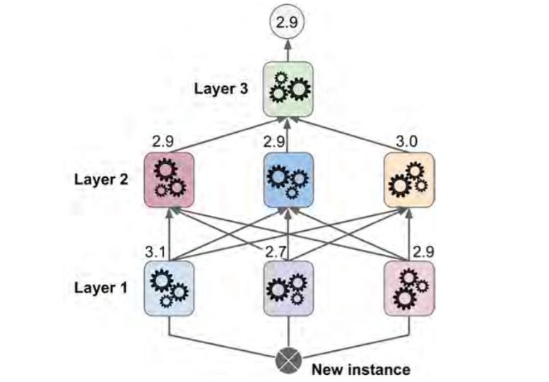
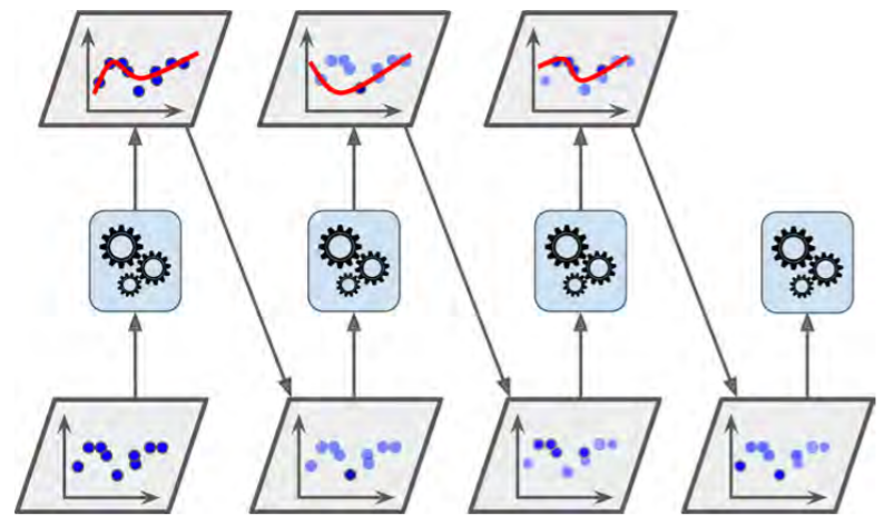
Stacking
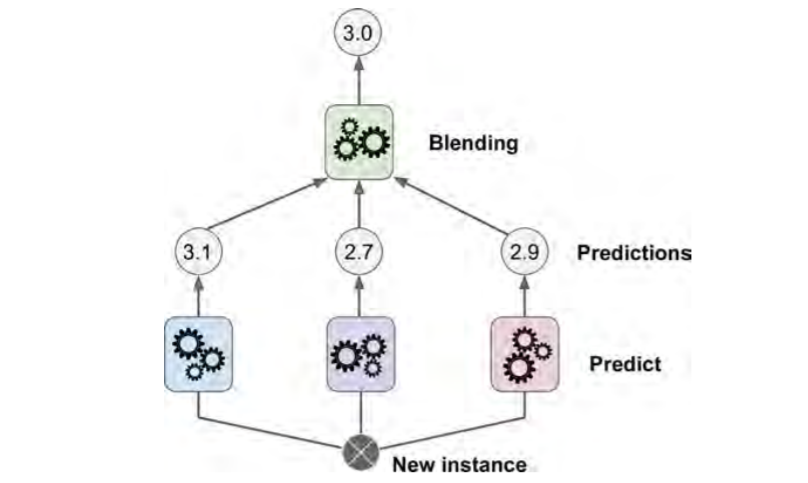
Stacked generalisation:It is based on a simple idea: instead of using trivial functions (such as hard voting) to aggregate the predictions of all predictors in an ensemble, why don’t we train a model to perform this aggregation?
Split Training Set into 2 and train layer 1 based on subset 1
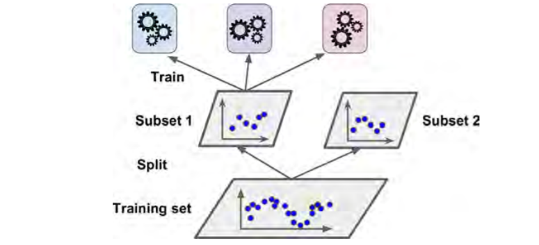
Train layer 2 based on predictions by layer 1 based on subset 2
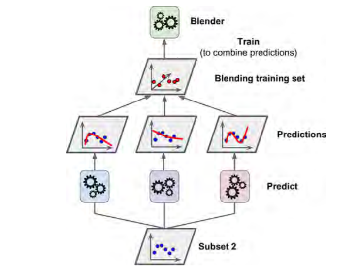
Final model