Training Models 2

Contents

SVM-Support Vector Machines

“Support Vector Machine” (SVM) is a supervised machine learning algorithm which can be used for either classification or regression problems. However, it is mostly used in classification. In this algorithm, we plot each data item as a point in n-dimensional space (where n is the number of features you have) called support vectors. Then, we perform classification by finding the hyperplane that differentiates the two classes. Additionally, SVM is robust to outliers and has a feature to ignore them.

SVM constructs a hyperplane in multidimensional space to separate different classes. SVM generates optimal hyperplane in an iterative manner, which is used to minimize an error. The core idea of SVM is to find a maximum marginal hyperplane(MMH) that best divides the dataset into classes.

• ref (https://engmrk.com/module-16-support-vector-machine-2/?utm_campaign=News&utm_medium=Community&utm_source=DataCamp.com_)
• (https://datacamp.com/community/tutorials/svm-classification-scikit-learn-python)

Support Vectors

• Support vectors are the data points, which are closest to the hyperplane. These points will define the separating line better by calculating margins. These points are more relevant to the construction of the classifier.

Hyperplane

• A hyperplane is a decision plane which separates between a set of objects having different class memberships.
• Plane which is of n-1 dimension where n is dimension of data.

Margin

• A margin is a gap between the two lines on the closest class points. This is calculated as the perpendicular distance from the line to support vectors or closest points. If the margin is larger in between the classes, then it is considered a good margin, a smaller margin is a bad margin.

How does SVM work?

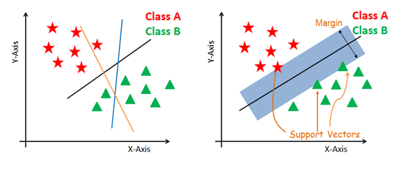
The main objective is to segregate the given dataset in the best possible way. The distance between the either nearest points is known as the margin. The objective is to select a hyperplane with the maximum possible margin between support vectors in the given dataset. SVM searches for the maximum marginal hyperplane in the following steps:

1. Generate hyperplanes which segregates the classes in the best way. Left-hand side figure showing three hyperplanes black, blue and orange. Here, the blue and orange have higher classification error, but the black is separating the two classes correctly.

2. Select the right hyperplane with the maximum segregation from the either nearest data points as shown in the right-hand side figure.

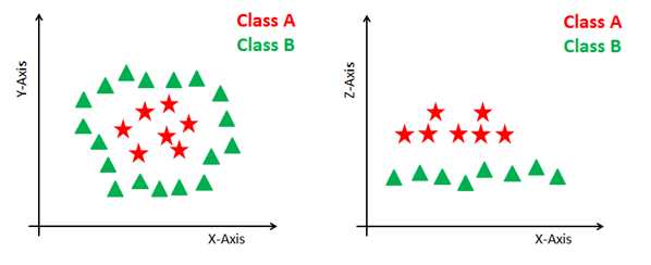
Dealing with non-linear and inseparable planes Some problems can’t be solved using linear hyperplane, as shown in the figure below (left-hand side).

In such situation, SVM uses a kernel trick to transform the input space to a higher dimensional space as shown on the right. The data points are plotted on the x-axis and z-axis (Z is the squared sum of both x and y: z=x^2=y^2). Now you can easily segregate these points using linear separation.

Types of SVM kernels

• Linear Kernel:A linear kernel can be used as normal dot product any two given observations. The product between two vectors is the sum of the multiplication of each pair of input values.

• Polynomial Kernel:A polynomial kernel is a more generalized form of the linear kernel. The polynomial kernel can distinguish curved or nonlinear input space

• Radial Basis Function Kernel: The Radial basis function kernel is a popular kernel function commonly used in support vector machine classification. RBF can map an input space in infinite dimensional space

SVM Parameters

• C

• C is used during the training phase and says how much outliers are taken into account in calculating Support Vectors.

• A low C makes the decision surface smooth, while a high C aims at classifying all training examples correctly by giving the model freedom to select more samples as support vectors.

• Gamma

• The gamma parameter defines how far the influence of a single training example reaches, with low values meaning ‘far’ and high values meaning ‘close’.

• The gamma parameters can be seen as the inverse of the radius of influence of samples selected by the model as support vectors.

• Kernel

• This parameter has many options like, “linear”, “rbf”,”poly” and others (default value is “rbf”). ‘linear’ is used for linear hyper-plane whereas “rbf” and “poly” are used for non-linear hyper-plane.

Soft Margin Classification

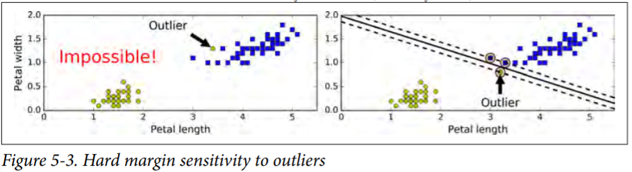
If we strictly impose that all instances be off the street and on the right side, this is called hard margin classification. There are two main issues with hard margin classification.

• it only works if the data is linearly separable.
• it is quite sensitive to outliers.

To avoid these issues it is preferable to use a more flexible model. The objective is to find a good balance between keeping the street as large as possible and limiting the margin violations (i.e., instances that end up in the middle of the street or even on the wrong side). This is called soft margin classification.

In Scikit-Learn’s SVM classes, you can control this balance using the C hyperparameter: a smaller C value leads to a wider street but more margin violations.

import numpy as np
from sklearn import datasets
from sklearn.pipeline import Pipeline
from sklearn.preprocessing import StandardScaler
from sklearn.svm import LinearSVC
iris = datasets.load_iris()
X = iris["data"][:, (2, 3)] # petal length, petal width
y = (iris["target"] == 2).astype(np.float64) # Iris-Virginica
svm_clf = Pipeline((
 ("scaler", StandardScaler()),
 ("linear_svc", LinearSVC(C=1, loss="hinge")),
 ))
svm_clf.fit(X, y)

Pipeline(memory=None,
         steps=[('scaler',
                 StandardScaler(copy=True, with_mean=True, with_std=True)),
                ('linear_svc',
                 LinearSVC(C=1, class_weight=None, dual=True,
                           fit_intercept=True, intercept_scaling=1,
                           loss='hinge', max_iter=1000, multi_class='ovr',
                           penalty='l2', random_state=None, tol=0.0001,
                           verbose=0))],
         verbose=False)

svm_clf.predict([[5.5, 1.7]])

array([1.])

• using SVC(kernel="linear", C=1) is also possible, but it is much slower, especially with large training sets, so it is not recommended.
• The SGDClassifier class, with SGDClassifier(loss="hinge",alpha=1/(m*C)). This applies regular Stochastic Gradient Descent to train a linear SVM classifier. It does not converge as fast as the LinearSVC class, but it can be useful to handle huge datasets that do not fit in memory (out-of-core training), or to handle online classification tasks.

The LinearSVC class regularizes the bias term, so you should center the training set first by subtracting its mean. This is automatic if you scale the data using the StandardScaler. Moreover, make sure you set the loss hyperparameter to "hinge", as it is not the default value. Finally, for better performance you should set the dual hyperparameter to False, unless there are more features than training instances

Nonlinear SVM Classification

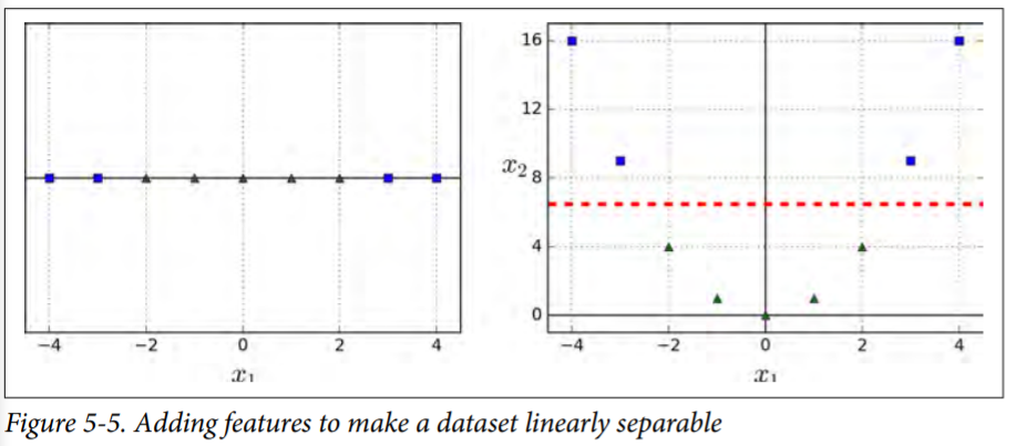
Although linear SVM classifiers are efficient and work surprisingly well in many cases, many datasets are not even close to being linearly separable. One approach to handling nonlinear datasets is to add more features, such as polynomial features.

Consider the left plot in Figure it represents a simple dataset with just one feature x1. This dataset is not linearly separable, as you can see. But if you add a second feature $x_2 = (x_1)^2$, the resulting 2D dataset is perfectly linearly separable.

from sklearn.datasets import make_moons
from sklearn.pipeline import Pipeline
from sklearn.preprocessing import PolynomialFeatures
polynomial_svm_clf = Pipeline((
 ("poly_features", PolynomialFeatures(degree=3)),
 ("scaler", StandardScaler()),
 ("svm_clf", LinearSVC(C=10, loss="hinge"))
 ))
polynomial_svm_clf.fit(X, y)

Polynomial Kernel

Adding polynomial features is simple to implement and can work great with all sorts of Machine Learning algorithms (not just SVMs), but at a low polynomial degree it cannot deal with very complex datasets, and with a high polynomial degree it creates a huge number of features, making the model too slow. Fortunately, when using SVMs you can apply an almost miraculous mathematical technique called the kernel trick (it is explained in a moment). It makes it possible to get the same result as if you added many polynomial features, even with very highdegree polynomials, without actually having to add them. So there is no combinatorial explosion of the number of features since you don’t actually add any features. This trick is implemented by the SVC class.

from sklearn.svm import SVC
poly_kernel_svm_clf = Pipeline((
 ("scaler", StandardScaler()),
 ("svm_clf", SVC(kernel="poly", degree=3, coef0=1, C=5))
 ))
poly_kernel_svm_clf.fit(X, y)

A common approach to find the right hyperparameter values is to use grid search. It is often faster to first do a very coarse grid search, then a finer grid search around the best values found. Having a good sense of what each hyperparameter actually does can also help you search in the right part of the hyperparameter space.

Adding Similarity Features

Another technique to tackle nonlinear problems is to add features computed using a similarity function that measures how much each instance resembles a particular landmark.

let’s define the similarity function to be the Gaussian Radial Basis Function (RBF) with γ = 0.3

$$ Gaussian RBF $$$$\phi y(x,l)=exp(-y|x-l|^2)$$

Gaussian RBF Kernel

Just like the polynomial features method, the similarity features method can be useful with any Machine Learning algorithm, but it may be computationally expensive to compute all the additional features, especially on large training sets. However, once again the kernel trick does its SVM magic: it makes it possible to obtain a similar result as if you had added many similarity features, without actually having to add them.

rbf_kernel_svm_clf = Pipeline((
 ("scaler", StandardScaler()),
 ("svm_clf", SVC(kernel="rbf", gamma=5, C=0.001))
 ))
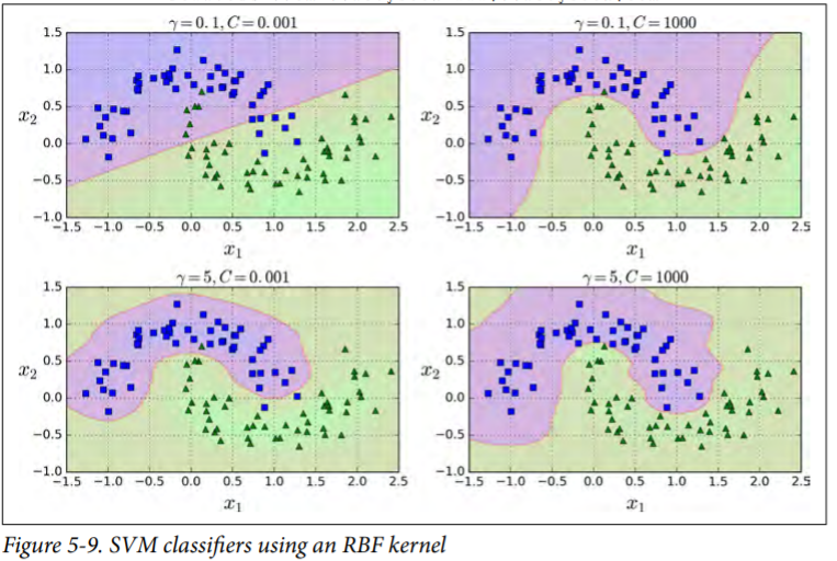
rbf_kernel_svm_clf.fit(X, y)

This model is represented on the bottom left of Figure. The other plots show models trained with different values of hyperparameters gamma (γ) and C. Increasing gamma makes the bell-shape curve narrower , and as a result each instance’s range of influence is smaller: the decision boundary ends up being more irregular, wiggling around individual instances. Conversely, a small gamma value makes the bell-shaped curve wider, so instances have a larger range of influence, and the decision boundary ends up smoother. So γ acts like a regularization hyperparameter: if your model is overfitting, you should reduce it, and if it is underfitting, you should increase it (similar to the C hyperparameter).

IMPORTANT

With so many kernels to choose from, how can you decide which one to use? As a rule of thumb, you should always try the linear kernel first (remember that LinearSVC is much faster than SVC(ker nel="linear")), especially if the training set is very large or if it has plenty of features. If the training set is not too large, you should try the Gaussian RBF kernel as well; it works well in most cases. Then if you have spare time and computing power, you can also experiment with a few other kernels using cross-validation and grid search, especially if there are kernels specialized for your training set’s data structure

Computational Complexity

SVM Regression

from sklearn.svm import LinearSVR
svm_reg = LinearSVR(epsilon=1.5)
svm_reg.fit(X, y)

from sklearn.svm import LinearSVR
svm_reg = LinearSVR(epsilon=1.5)
svm_reg.fit(X, y)

Add Under The Hood Theory for SVM

Class	Time complexity	Out-of-core support	Scaling required	Kernel trick
LinearSVC	O(m × n)	No	Yes	No
SGDClassifier	O(m × n)	Yes	Yes	No
SVC	O(m² × n) to O(m³ × n)	No	Yes	Yes