Linear Regression
Equation 4-1. Linear Regression model prediction
$y = θ_{0} + θ_{1}x_{1} + θ_{2}x_{2} + ⋯ + θ_{n}x_{n}$
- ŷ is the predicted value.
- n is the number of features.
- $x_{i}$ is the ith feature value.
- $θ_{j}$ is the jth model parameter (including the bias term $θ_{0}$ and the feature weights $θ_{1} , θ_{2} , ⋯, θ_{n})$.
Equation 4-2. Linear Regression model prediction (vectorized form)
$y = hθ(x) = θ^{T}.x$
we use MSE cost Function and then minimise it.
$MSE (x , hθ) = \frac{∑(θ^{T}·x(i)− y(i))^2}{m}$
One way to do this is to use Normal Equation which directly gives us values of theta
$θ = ((X^{T}·X)^{-1}).X^{T}.y$
import numpy as np
import seaborn as sns
X=np.arange(100)
delta = np.random.uniform(-36,36, size=(100,))
y=4+3*X+delta
sns.scatterplot(data=y)
X_b=np.c_[np.ones((100,1)),X]
theta_best=np.linalg.inv(X_b.T.dot(X_b)).dot(X_b.T).dot(y)
theta_best
X_new = np.arange(100)
X_new_b = np.c_[np.ones((100, 1)), X_new] # add x0 = 1 to each instance
y_predict = X_new_b.dot(theta_best)
import matplotlib.pyplot as plt
plt.plot( y_predict, "r-")
plt.plot( y, "c.")
plt.show()

The Normal Equation gets very slow when the number of features grows large (e.g., 100,000).
The Normal Equation computes the inverse of $X^{T} · X$, which is an n × n matrix (where n is the number of features). The computational complexity of inverting such a matrix is typically about O(n 2.4) to O(n 3 ) (depending on the implementation). In other words, if you double the number of features, you multiply the computation time by roughly 22.4 = 5.3 to 23 = 8.
On the positive side, this equation is linear with regards to the number of instances in the training set (it is O(m)), so it handles large training sets efficiently, provided they can fit in memory.
Gradient Descent
Gradient Descent is a very generic optimization algorithm capable of finding optimal solutions to a wide range of problems.
The general idea of Gradient Descent is to tweak parameters iteratively in order to minimize a cost function.you start by filling θ with random values (this is called random initializa‐ tion), and then you improve it gradually, taking one baby step at a time, each step attempting to decrease the cost function (e.g., the MSE), until the algorithm converges to a minimum.
An important parameter in Gradient Descent is the size of the steps, determined by the learning rate hyperparameter. If the learning rate is too small, then the algorithm will have to go through many iterations to converge, which will take a long time. On the other hand, if the learning rate is too high, you might jump across the valley and end up on the other side, possibly even higher up than you were before. This might make the algorithm diverge, with larger and larger values, failing to find a good solution
When using Gradient Descent, you should ensure that all features have a similar scale (e.g., using Scikit-Learn’s StandardScaler class), or else it will take much longer to converge.
Batch Gradient Descent
Code not Working
probably not working because gradient descent requires scaled data and this is not scaled?
X=np.arange(100)
delta = np.random.uniform(-36,36,100)
y=4+3*X+delta
y=y.reshape((100,1))
sns.scatterplot(data=y)
X_b=np.c_[np.ones((100,1)),X]
eta = 0.1 # learning rate
n_iterations = 100
m = 100
theta = np.random.randn(2,1)+16
print(theta)# random initialization
# print(X_b.shape)
# print(X_b.T.shape)
# print(theta.shape)
# print(y.shape)
# print((np.subtract(np.dot(X_b,theta),y)).shape)
for iteration in range(n_iterations):
    gradients = 2/m*X_b.T.dot(X_b.dot(theta)-y)
    #print(gradients.shape)
    theta = theta + eta*gradients

theta
Stochastic Gradient Descent
- The main problem with Batch Gradient Descent is the fact that it uses the whole training set to compute the gradients at every step, which makes it very slow when the training set is large. At the opposite extreme, Stochastic Gradient Descent just picks a random instance in the training set at every step and computes the gradients based only on that single instance. Obviously this makes the algorithm much faster since it has very little data to manipulate at every iteration. It also makes it possible to train on huge training sets, since only one instance needs to be in memory at each iteration (SGD can be implemented as an out-of-core algorithm.)
- On the other hand, due to its stochastic (i.e., random) nature, this algorithm is much less regular than Batch Gradient Descent: instead of gently decreasing until it reaches the minimum, the cost function will bounce up and down, decreasing only on average. Over time it will end up very close to the minimum, but once it gets there it will continue to bounce around, never settling down
X_b=X_b.reshape(100,2)
y=y.reshape(100,1)
from sklearn.linear_model import SGDRegressor
sgd_reg = SGDRegressor(penalty=None, eta0=0.1)
sgd_reg.fit(X, y.ravel())
Mini-batch Gradient Descent
- Mini-batch GD computes the gradients on small random sets of instances called minibatches
- The main advantage of Mini-batch GD over Stochastic GD is that you can get a performance boost from hardware optimization of matrix operations, especially when using GPUs.
print("""
Algorithm           Large m     Out-of-core support      Large n     Hyperparams     Scaling required      Scikit-Learn
Normal Equation     Fast        No                       Slow        0               No                    n/a
Batch GD            Slow        No                       Fast        2               Yes                   SGDRegressor
Stochastic GD       Fast        Yes                      Fast        ≥2              Yes                   SGDRegressor
Mini-batch GD       Fast        Yes                      Fast        ≥2              Yes                   SGDRegressor
SVD                 Fast        No                       Slow        0               No                    LinearRegression
""")
Polynomial Regression
What if your data is actually more complex than a simple straight line? Surprisingly, you can actually use a linear model to fit nonlinear data. A simple way to do this is to add powers of each feature as new features, then train a linear model on this extended set of features. This technique is called Polynomial Regression.
m = 100
X = np.arange(-100,100).reshape(200,1)
y = 0.5 * X**2 + X + 2 + 700*np.random.randn(200,1)
sns.scatterplot(data=y)

from sklearn.preprocessing import PolynomialFeatures
from sklearn.linear_model import LinearRegression
poly_features = PolynomialFeatures(degree=2, include_bias=False)
X_poly = poly_features.fit_transform(X)
lin_reg = LinearRegression()
lin_reg.fit(X_poly, y)
lin_reg.intercept_, lin_reg.coef_
 # add x0 = 1 to each instance
y_predict = lin_reg.predict(X_poly)
plt.plot( y_predict, "r-")
plt.plot(y,"c.")
plt.show()

Examples of Overfitting
poly_features = PolynomialFeatures(degree=20, include_bias=False)
X_poly = poly_features.fit_transform(X)
lin_reg = LinearRegression()
lin_reg.fit(X_poly, y)
lin_reg.intercept_, lin_reg.coef_
y_predict = lin_reg.predict(X_poly)
plt.plot( y_predict, "r-")
plt.plot(y,"c.")
plt.show()

using pipelining for polynomial regression
from sklearn.pipeline import Pipeline
polynomial_regression = Pipeline((
 ("poly_features", PolynomialFeatures(degree=10, include_bias=False)),
 ("sgd_reg", LinearRegression()),
 ))
plot_learning_curves(polynomial_regression, X, y)
from sklearn.metrics import mean_squared_error
from sklearn.model_selection import train_test_split
from sklearn.preprocessing import PolynomialFeatures
from sklearn.linear_model import LinearRegression
import matplotlib.pyplot as plt
import numpy as np

def plot_learning_curves(model, X, y):
    X_train, X_val, y_train, y_val = train_test_split(X, y, test_size=0.2)
    train_errors, val_errors = [], []
    for m in range(1, len(X_train)):
        model.fit(X_train[:m], y_train[:m])
        y_train_predict = model.predict(X_train[:m])
        y_val_predict = model.predict(X_val)
        train_errors.append(mean_squared_error(y_train_predict, y_train[:m]))
        val_errors.append(mean_squared_error(y_val_predict, y_val))
    plt.plot(np.sqrt(train_errors), "r-+", linewidth=2, label="train")
    plt.plot(np.sqrt(val_errors), "b-", linewidth=3, label="val")

X = np.arange(-100,100).reshape(200,1)
y = 0.5 * X**2 + X + 2 + 700*np.random.randn(200,1)

poly_features = PolynomialFeatures(degree=2, include_bias=False)
X_poly = poly_features.fit_transform(X)
lin_reg = LinearRegression()
plot_learning_curves(lin_reg, X_poly, y)
plt.legend()

- One way to improve an overfitting model is to feed it more training data until the validation error reaches the training error
The Bias/Variance Tradeoff
- a model’s generalization error can be expressed as the sum of three very different errors:
Bais
- This part of the generalization error is due to wrong assumptions, such as assum‐ ing that the data is linear when it is actually quadratic. A high-bias model is most likely to underfit the training data.
Variance
- This part is due to the model’s excessive sensitivity to small variations in the training data. A model with many degrees of freedom (such as a high-degree polynomial model) is likely to have high variance, and thus to overfit the training data
Irreducible error
- This part is due to the noisiness of the data itself. The only way to reduce this part of the error is to clean up the data (e.g., fix the data sources, such as broken sensors, or detect and remove outliers)
Regularuized Linear Models
Ridge Regression
Ridge Regression (also called Tikhonov regularization) is a regularized version of Linear Regression: a regularization term equal to $α∑θ(i)^{2}$ is added to the cost function. This forces the learning algorithm to not only fit the data but also keep the model weights as small as possible. Note that the regularization term should only be added to the cost function during training. Once the model is trained, you want to evaluate the model’s performance using the unregularized performance measure.
It is important to scale the data (e.g., using a StandardScaler) before performing Ridge Regression, as it is sensitive to the scale of the input features. This is true of most regularized models
$J(θ)=MSE(θ)+α*0.5*∑θ(i)^{2}$
Ridge Regression Closed Form
$θ = ((X^{T}·X + αA)^{-1})·X^{T}·Y$
A is the n × n identity matrix except with a 0 in the top-left cell, corresponding to the bias term
code example
from sklearn.linear_model import Ridge
ridge_reg = Ridge(alpha=1, solver="cholesky")
ridge_reg.fit(X, y)
ridge_reg.predict([[1.5]])
sgd_reg = SGDRegressor(penalty="l2")
sgd_reg.fit(X, y.ravel())
sgd_reg.predict([[1.5]])
In layman terms using ridge regression flattens the prediction line. write code to check this for yourself. plot prediction line for different values of alpha
Lasso Regression
Least Absolute Shrinkage and Selection Operator Regression (simply called Lasso Regression) is another regularized version of Linear Regression: just like Ridge Regression, it adds a regularization term to the cost function, but it uses the ℓ1 norm of the weight vector instead of half the square of the ℓ2 norm
$J(θ) = MSE(θ) + α∑|θ_{i}|$
An important characteristic of Lasso Regression is that it tends to completely eliminate the weights of the least important features (i.e., set them to zero).
from sklearn.linear_model import Lasso
lasso_reg = Lasso(alpha=0.1)
lasso_reg.fit(X, y)
lasso_reg.predict([[1.5]])
Elastic Net
Elastic Net is a middle ground between Ridge Regression and Lasso Regression. The regularization term is a simple mix of both Ridge and Lasso’s regularization terms, and you can control the mix ratio r. When r = 0, Elastic Net is equivalent to Ridge Regression, and when r = 1, it is equivalent to Lasso Regression
$J(θ) = MSE(θ) + rα∑|θ_{i}| + (\frac{(1 − r)}{2})*α∑(θ_{i})^{2}$
from sklearn.linear_model import ElasticNet
elastic_net = ElasticNet(alpha=0.1, l1_ratio=0.5)
elastic_net.fit(X, y)
elastic_net.predict([[1.5]])
Important(when to use what kind Of regression)
It is almost always preferable to have at least a little bit of regularization, so generally you should avoid plain Linear Regression. Ridge is a good default, but if you suspect that only a few features are actually useful, you should prefer Lasso or Elastic Net since they tend to reduce the useless features’ weights down to zero as we have discussed. In general, Elastic Net is preferred over Lasso since Lasso may behave erratically when the num‐ ber of features is greater than the number of training instances or when several fea‐ tures are strongly correlated.
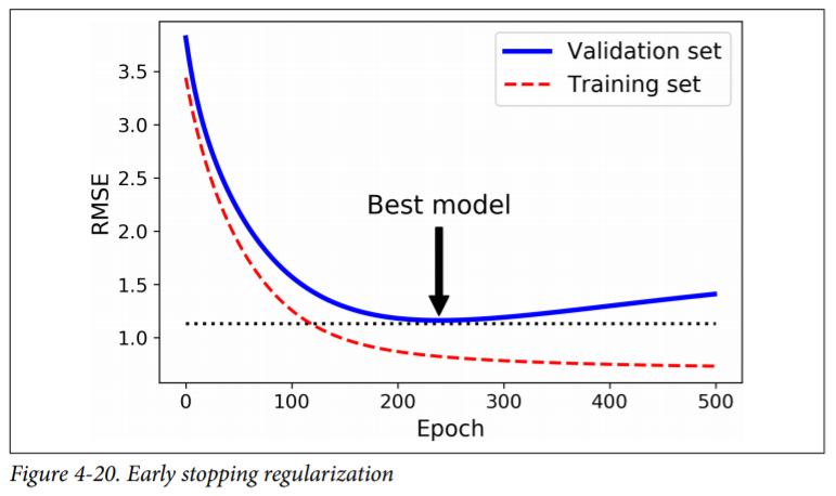
Early Stopping
A very different way to regularize iterative learning algorithms such as Gradient Descent is to stop training as soon as the validation error reaches a minimum. This is called early stopping.
Figure 4-20 shows a complex model (in this case a high-degree Polynomial Regression model) being trained using Batch Gradient Descent. As the epochs go by, the algorithm learns and its prediction error (RMSE) on the training set naturally goes down, and so does its prediction error on the validation set. However, after a while the validation error stops decreasing and actually starts to go back up. This indicates that the model has started to overfit the training data. With early stop‐ ping you just stop training as soon as the validation error reaches the minimum. It is such a simple and efficient regularization technique that Geoffrey Hinton called it a “beautiful free lunch.”
Basic Implementation
from sklearn.base import clone
# prepare the data
poly_scaler = Pipeline([
 ("poly_features", PolynomialFeatures(degree=90, include_bias=False)),
 ("std_scaler", StandardScaler())
 ])
X_train_poly_scaled = poly_scaler.fit_transform(X_train)
X_val_poly_scaled = poly_scaler.transform(X_val)
sgd_reg = SGDRegressor(max_iter=1, tol=-np.infty, warm_start=True,
 penalty=None, learning_rate="constant", eta0=0.0005)
minimum_val_error = float("inf")
best_epoch = None
best_model = None
for epoch in range(1000):
    sgd_reg.fit(X_train_poly_scaled, y_train) # continues where it left off
    y_val_predict = sgd_reg.predict(X_val_poly_scaled)
    val_error = mean_squared_error(y_val, y_val_predict)
    if val_error < minimum_val_error:
        minimum_val_error = val_error
        best_epoch = epoch
        best_model = clone(sgd_reg)
Logistic Regression
Logistic Regression (also called Logit Regression) is commonly used to estimate the probability that an instance belongs to a particular class (e.g., what is the probability that this email is spam?). If the estimated probability is greater than 50%, then the model predicts that the instance belongs to that class (called the positive class, labeled “1”), or else it predicts that it does not (i.e., it belongs to the negative class, labeled “0”). This makes it a binary classifier.
Just like a Linear Regression model, a Logistic Regression model computes a weighted sum of the input features (plus a bias term), but instead of outputting the result directly like the Linear Regression model does, it outputs the logistic of this result
Logistic Regression model estimated probability (vectorized form)
$p = hθ(x) = σ(θ^{T}.x)$
The logistic—also called the logit, noted σ(·)—is a sigmoid function (i.e., S-shaped) that outputs a number between 0 and 1.
Sigmoid Function
x=np.arange(-10,10).reshape(20,1)
sigma = 1/(1+np.exp(-1*x))
plt.figure(figsize=(20,6))
sns.set_style("whitegrid")
sns.lineplot(data=sigma)

Logistic Regression cost function (log loss)
$J(θ)= \frac{−1}{m}∑(y(i)log(p(i))+ (1 − y(i))log( 1 − p(i))$
Logistic cost function partial derivatives
$(\frac{∂}{∂θj})(J(θ)) = (1/m) ∑ (σ(θ^{T}·x(i))− y(i))x_{j}(i)$
from sklearn import datasets
import numpy as np
iris=datasets.load_iris()
list(iris.keys())
x=iris["data"][:,3:]
y=(iris["target"]==2).astype(np.int)
from sklearn.linear_model import LogisticRegression
log_reg=LogisticRegression()
log_reg.fit(x,y)
X_new=np.linspace(0,3,1000).reshape(-1,1)
y_proba=log_reg.predict_proba(X_new)
import matplotlib.pyplot as plt
plt.figure(figsize=(20,6))
plt.plot(X_new,y_proba[:,1],"g-",label="Iris-Virginica")
plt.plot(X_new,y_proba[:,0],"b--",label="Not Iris-Virginica")
plt.legend()
plt.show()

Softmax Regression
The Logistic Regression model can be generalized to support multiple classes directly, without having to train and combine multiple binary classifiers This is called Softmax Regression, or Multinomial Logistic Regression.
Softmax score for class k
$sk(x) = θ_{k}^{T}·x$
Cross Entropy
Cross entropy originated from information theory. Suppose you want to efficiently transmit information about the weather every day. If there are eight options (sunny, rainy, etc.), you could encode each option using 3 bits since 23 = 8. However, if you think it will be sunny almost every day, it would be much more efficient to code “sunny” on just one bit (0) and the other seven options on 4 bits (starting with a 1). Cross entropy measures the average number of bits you actually send per option. If your assumption about the weather is perfect, cross entropy will just be equal to the entropy of the weather itself (i.e., its intrinsic unpredictability). But if your assump‐ tions are wrong (e.g., if it rains often), cross entropy will be greater by an amount called the Kullback–Leibler divergence. The cross entropy between two probability distributions p and q is defined as H p, q = − ∑x p x log q x (at least when the distributions are discrete).
Decision Trees
Decision Trees are versatile Machine Learning algorithms that can per‐ form both classification and regression tasks, and even multioutput tasks
# sklearn example for iris dataset w Decision Tree

from sklearn.datasets import load_iris
from sklearn.tree import DecisionTreeClassifier
iris = load_iris()
X = iris.data[:, 2:] # petal length and width
y = iris.target
tree_clf = DecisionTreeClassifier(max_depth=2)
tree_clf.fit(X, y)
tree_clf.score(X,y)
We can export Decision Tree graphs by using export_graphviz
from sklearn import tree
from graphviz import Source
graph = Source(tree.export_graphviz(tree_clf, out_file="iris_tree.dot"
   , feature_names=iris.feature_names[2:], class_names=iris.target_names,
   rounded=True, filled = True))
# display(SVG(graph.pipe(format='svg')))
from sklearn.tree import export_graphviz
export_graphviz(
 tree_clf,
 out_file=image_path("iris_tree.dot"),
 feature_names=iris.feature_names[2:],
 class_names=iris.target_names,
 rounded=True,
 filled=True
 )
Use graphviz to convert following to png image using the following command in command line
dot -Tpng iris_tree.dot -o iris_tree.png
One of the many qualities of Decision Trees is that they require very little data preparation. In particular, they don’t require feature scaling or centering at all.
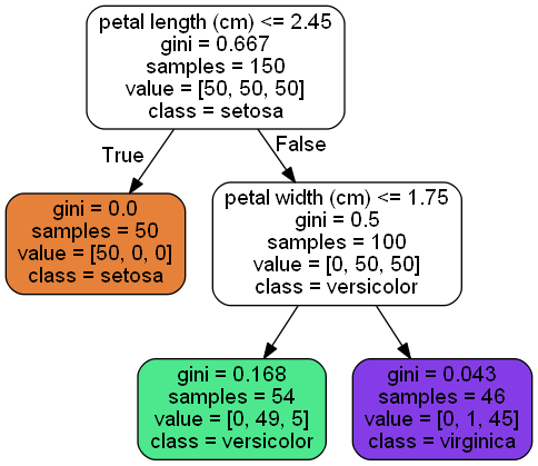
A node’s gini attribute measures its impur‐ ity: a node is “pure” (gini=0) if all training instances it applies to belong to the same class. For example, since the depth-1 left node applies only to Iris-Setosa training instances, it is pure and its gini score is 0.
$Gi = 1 − ∑(pi, k^{2})$
- pi,k is the ratio of class k instances among the training instances in the $i^{th}$ node
Scikit-Learn uses the CART algorithm, which produces only binary trees: nonleaf nodes always have two children (i.e., questions only have yes/no answers). However, other algorithms such as ID3 can produce Decision Trees with nodes that have more than two chil‐ dren.
Estimating Probabilities
A Decision Tree can also estimate the probability that an instance belongs to a partic‐ ular class k: first it traverses the tree to find the leaf node for this instance, and then it returns the ratio of training instances of class k in this node. For example, suppose you have found a flower whose petals are 5 cm long and 1.5 cm wide. The corre‐ sponding leaf node is the depth-2 left node, so the Decision Tree should output the following probabilities: 0% for Iris-Setosa (0/54), 90.7% for Iris-Versicolor (49/54), and 9.3% for Iris-Virginica (5/54). And of course if you ask it to predict the class, it should output Iris-Versicolor (class 1) since it has the highest probability.
tree_clf.predict_proba([[5,1.5]])
Model Interpretation: White Box Versus Black Box
As you can see Decision Trees are fairly intuitive and their decisions are easy to interpret. Such models are often called white box models. In contrast, as we will see, Random Forests or neural networks are generally considered black box models. They make great predictions, and you can easily check the calculations that they performed to make these predictions; nevertheless, it is usually hard to explain in simple terms why the predictions were made. For example, if a neural network says that a particular person appears on a picture, it is hard to know what actually contributed to this prediction: did the model recognize that person’s eyes? Her mouth? Her nose? Her shoes? Or even the couch that she was sitting on? Conversely, Decision Trees provide nice and simple classification rules that can even be applied manually if need be (e.g., for flower classification).
Under the Hood for Decision Tree
- Uses the Classification and Regression tree algorithm to train Decision trees;CART Training Algorithm.
- The idea is really quite simple: the algorithm first splits the training set in two subsets using a single feature k and a threshold tk.(e.g., “petal length ≤ 2.45 cm”). How does it choose k and tk ? It searches for the pair (k, tk) that produces the purest subsets (weighted by their size). The cost function is
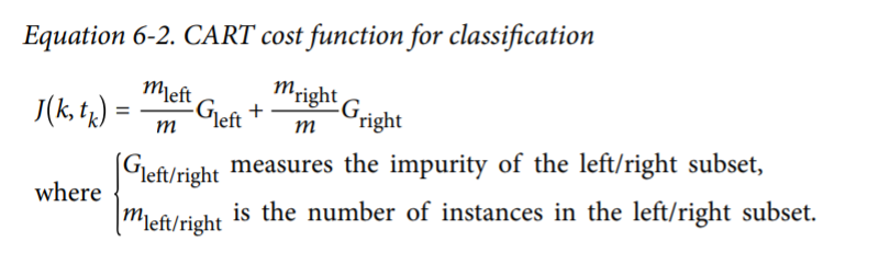
It stops recursing once it rea‐ ches the maximum depth (defined by the max_depth hyperparameter), or if it cannot find a split that will reduce impurity
the CART algorithm is a greedy algorithm: it greed‐ ily searches for an optimum split at the top level, then repeats the process at each level. It does not check whether or not the split will lead to the lowest possible impurity several levels down. A greedy algorithm often produces a reasonably good solution, but it is not guaranteed to be the optimal solution.
Regression
m = 100
X = np.arange(-100,100).reshape(200,1)
y = 0.5 * X**2 + X + 2 + 700*np.random.randn(200,1)
sns.scatterplot(data=y)

from sklearn.tree import DecisionTreeRegressor
tree_reg = DecisionTreeRegressor(max_depth=2)
tree_reg.fit(X,y)
y_new=tree_reg.predict(X)
Plot for Depth=2
import matplotlib.pyplot as plt
plt.plot(y,"c.")
plt.plot(y_new,"r-")

Plot for depth=10
Is this overfit? try increasing max_depth for clear idea
tree_reg2=DecisionTreeRegressor(max_depth=5)
tree_reg2.fit(X,y)
y_new2=tree_reg2.predict(X)
plt.plot(y,"c.")
plt.plot(y_new2,"r-")

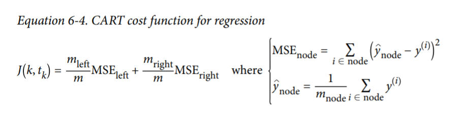
The CART algorithm works mostly the same way as earlier, except that instead of try‐ ing to split the training set in a way that minimizes impurity, it now tries to split the training set in a way that minimizes the MSE.
using a reularization Hyperparameter we can fit data better
tree_reg2=DecisionTreeRegressor(min_samples_leaf=10)
tree_reg2.fit(X,y)
y_new2=tree_reg2.predict(X)
plt.plot(y,"c.")
plt.plot(y_new2,"r-")

Regularization Hyperparameters
Decision Trees make very few assumptions about the training data (as opposed to lin‐ ear models, which obviously assume that the data is linear, for example). If left unconstrained, the tree structure will adapt itself to the training data, fitting it very closely, and most likely overfitting it. Such a model is often called a nonparametric model, not because it does not have any parameters (it often has a lot) but because the number of parameters is not determined prior to training, so the model structure is free to stick closely to the data. In contrast, a parametric model such as a linear model has a predetermined number of parameters, so its degree of freedom is limited, reducing the risk of overfitting (but increasing the risk of underfitting). To avoid overfitting the training data, you need to restrict the Decision Tree’s freedom during training. As you know by now, this is called regularization. The regularization hyperparameters depend on the algorithm used, but generally you can at least restrict the maximum depth of the Decision Tree. In Scikit-Learn, this is controlled by the max_depth hyperparameter (the default value is None, which means unlimited). Reducing max_depth will regularize the model and thus reduce the risk of overfitting. The DecisionTreeClassifier class has a few other parameters that similarly restrict the shape of the Decision Tree: min_samples_split (the minimum number of samples a node must have before it can be split), min_samples_leaf (the minimum num‐ ber of samples a leaf node must have), min_weight_fraction_leaf (same as min_samples_leaf but expressed as a fraction of the total number of weighted instances), max_leaf_nodes (maximum number of leaf nodes), and maxfeatures (maximum number of features that are evaluated for splitting at each node). Increas‐ ing min hyperparameters or reducing max_ hyperparameters will regularize the model.
Other algorithms work by first training the Decision Tree without restrictions, then pruning (deleting) unnecessary nodes. A node whose children are all leaf nodes is considered unnecessary if the purity improvement it provides is not statistically significant. Stan‐ dard statistical tests, such as the χ 2 test, are used to estimate the probability that the improvement is purely the result of chance (which is called the null hypothesis). If this probability, called the pvalue, is higher than a given threshold (typically 5%, controlled by a hyperparameter), then the node is considered unnecessary and its children are deleted. The pruning continues until all unnecessary nodes have been pruned.
Instability
- Decision Trees love orthogonal decision boundaries (all splits are perpendicular to an axis), which makes them sensitive to training set rotation.
One way to limit this problem is to use PCA(Dimensionality reduction algorithm).
- Decision Trees is that they are very sensitive to small variations in the training data.
- the training algorithm used by Scikit-Learn is stochastic6 you may get very different models even on the same training data (unless you set the random_state hyperparameter).